7 Computational Modeling Concepts

In an attempt to robustly, and transparently, fit CPUT to behavioral data, I follow the general guidelines presented in Robert Wilson and Anne Collins’s paper Ten simple rules for the computational modeling of behavioral data.^[36]At a high level, they state that computational modeling allows us to make better sense of behavioral data with mathematical models that may provide insight into mechanisms underlying behavior. Although the exact form of the models may differ, the basic process of assessing a model’s descriptive and predictive efficacy is similar.

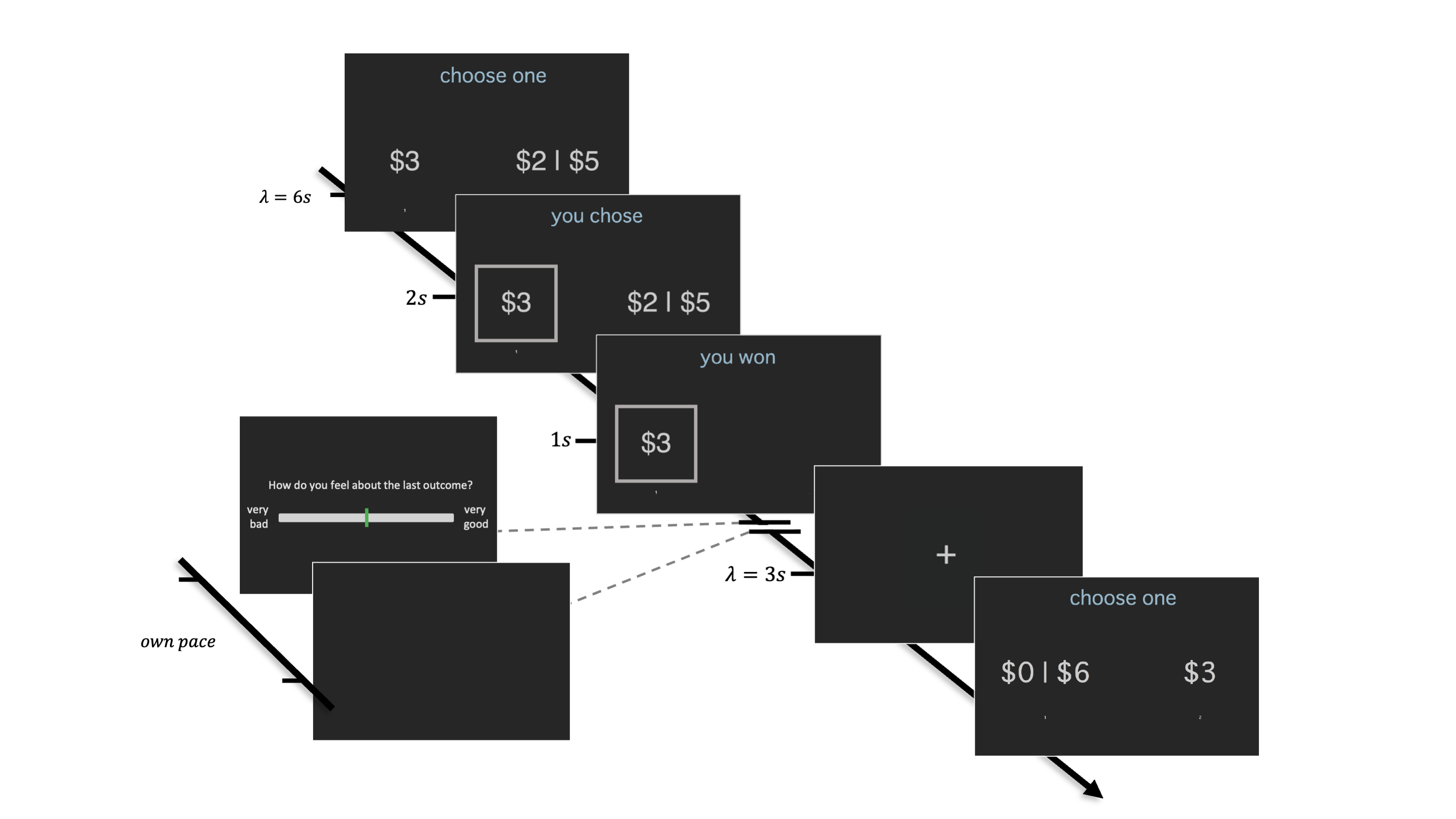
The first two steps Wilson and Collins discuss are designing an experiment and developing a model. For my thesis, I fit CPUT with data collected from an ongoing study by Brittany Liebenow and colleagues^[35] where forty-five healthy adults (ages 18-65) were recruited to complete a sure-bet or gamble task (Figure 7.1).

Figure 7.1: Schematic of a trial from the Sure Bet or Gamble task and subjective rating prompt. A prospect is presented for a random duration based on a Poisson distribution \((\lambda = 6\text{s})\). Assuming a timely response, a choice screen was shown for two seconds followed by an outcome screen for one second. Trials were separated with a fixation cross whose inter-trial interval was a random duration from a Poisson distribution with \(\lambda = 3\text{s}\).

For thirty minutes, participants indicated their preference for a sure bet (values between $1-$6 in $1 increments) or a fifty-fifty gamble between two non-identical values ($0 - $6 in $1 increments). The lateral presentation of the sure bet and gambles were randomized, and each prospect was presented for a random duration based on a Poisson distribution \((\lambda = 6\text{s})\). If the participant answered within the allotted time, their choice was displayed for two seconds before they were shown the outcome for one second. If they did not answer in time, they were shown a late screen for one second. Rounds were separated with a fixation cross whose inter-trial interval was a Poisson distribution \((\lambda = 6\text{s}\), zeros removed\()\). After one-third of of the rounds where choices were made, respondents were asked “How do you feel about the last outcome?” and could adjust a slider ranging from ‘very bad’ to ‘very good.’ Participants were paid $20 per hour and told they would receive winnings from a randomly selected round as bonus compensation.

Using this data from this task, we can group the remaining computational modeling steps into three stages:^[36]

• Simulation & Parameter Recovery: Use the candidate model (CPUT) to generate ‘fake’ behavioral data and attempt to recover the parameters of interest following the proposed analysis method for experimental data.

• Parameter Estimation: Find the set of parameters that best account for the experimental data given the candidate model.

• Model Comparison: Compare the candidate models to others (EUT) that may provide alternative explanations of the behavioral data.

Before detailing the methods and results for each stage in my analysis, it is important to understand the mathematics behind our model-fitting. In the remaining sections of this chapter, I discuss how Bayesian inference can help us infer from choice data the most plausible parameter values for a model.

7.1 Using Bayes’ Theorem to Estimate Parameters from Choice Behavior

Data from the sure bet or gamble task is represented as a binary variable. That is, for each prospect, if someone chose option one (the sure bet), we denote that with 1. Otherwise, it’s 0. and zero otherwise. For example, someone’s choice behavior for six prospects may look like this:

\[\begin{equation*} \begin{split} \text{Chose Option 1} = \begin{bmatrix} 0 \\ 1 \\ 1 \\ 1 \\ 1 \\ 0 \end{bmatrix} \end{split} \qquad \begin{split} \text{Chose Option 2} = \begin{bmatrix} 1 \\ 0 \\ 0 \\ 0 \\ 0 \\ 1 \end{bmatrix} \end{split} \end{equation*}\]

Given this binary choice behavior, the question becomes how we can estimate our parameter(s) of interest. And the answer is with Bayes’ Theorem! In the general case, Bayes’ Theorem states that the probability a parameter of interest, \(\theta\), is some value given the observed data is proportional to the likelihood of observing the data given that parameter value times the prior plausibility of the parameter being said value (Equation (7.1)).⁸

\[\begin{equation} \color{purple}{Pr(\theta|\text{Data})} \propto \color{maroon}{L(\text{Data}|\theta)} \times \color{royalblue}{\pi(\theta)} \tag{7.1} \end{equation}\]

We can rewrite Bayes’ Theorem in the context of estimating the counterfactual weighting term, \(\gamma\) from the human choice data. That is, the probability of \(\gamma\) being some value given the observed choices is proportional to the likelihood of observing a choice given that \(\gamma\) value times the prior plausibility of \(\gamma\) being that value (Equation (7.2)).

\[\begin{equation} \color{purple}{Pr(\gamma|\text{Choices})} \propto \color{maroon}{L(\text{Choice}|\gamma)} \times \color{RoyalBlue}{\pi(\gamma)} \tag{7.2} \end{equation}\]

In Bayesian inference, unknown parameters (e.g., \(\gamma\)) are considered as random variables from which we can relate to the observed data with a “likelihood function.^[38] The parameter of interest when assessing the descriptive and predictive validity of CPUT using human choice data is \(\gamma\). By defining the prior plausibility of \(\gamma\), I am able to incorporate existing information into my modeling.

Prior information may be influenced by previous experiments. Here, I make assumptions about the distribution of \(\gamma\) in light of the potential data-generating model, CPUT. Specifically, from the idea that people account for counterfactual information when making decisions, I assume that \(\gamma \ge 0\). I further assume people do not place more weight on counterfactual outcomes relative to factual ones. This constrains \(\gamma \le 1\). Together, the prior information I incorporate into my models suggests that values of \(0 \leq \gamma \leq 1\) are equally plausible. That is, \(\gamma\) is distributed from a uniform distribution between zero and one.

To refine the estimate of \(\gamma\) using Bayes’ Theorem, we need some way of defining the likelihood of observing a binary choice for a specific \(\gamma\) value. The likelihood describes the statistical model assumed to generate the choice behavior, relating the possible values for \(\gamma\) and the observed choices.^[38]

CPUT offers a way of determining utilities for a prospect’s options. In order to generate the data, we need some likelihood function that can transform these utilities into a valid statistical model. There are a number of these ‘action-selection’ methods^[15]. One common to both the psychological literature and the reinforcement learning field is the ‘soft-max’ choice rule: a logistic transformation of the difference in utilities for each option (Equation (7.3)).^[39] This introduces an additional parameter, \(\tau > 0\), that relates how sensitive one’s choice is to a difference in utilities. In the limit, as \(\tau \rightarrow \infty\), the probability of choosing the option with a higher utility approaches 1.

\[\begin{equation} \begin{aligned} L_{\text{Softmax}}(\text{Chose Option 1} | U_1, U_2, \tau) &= \frac{1}{1 + e^{(-\tau \cdot (U_1 - U_2))}} \\ L_{\text{Softmax}}(\text{Chose Option 2} | U_1, U_2, \tau) &= \frac{1}{1 + e^{(-\tau \cdot (U_2 - U_1))}} \end{aligned} \tag{7.3} \end{equation}\]

For my analysis, I used the softmax transformation as the likelihood function to relate the probability of choosing option one, the sure bet, with \(\gamma\). That is, the mathematical description of the model I used to assess CPUT’s veracity, represented in Equation (7.4), says:

• An individual choice for option 1 is made with probability \(p\), where
• \(p\) is determined through a softmax transformation of the counterfactual utilities for each option, \(U_{C1}(\gamma), U_{C2}(\gamma)\), and a sensitivity parameter, \(\tau\), where
• \(\tau\) is assumed to be uniform between zero and thirty, and
• \(\gamma\) is assumed to be uniform between zero and one.

\[\begin{equation} \begin{aligned} \text{Chose Option 1} &\sim \text{Bernoulli}(p) \\ p &= L_{\text{Softmax}}\Big(\text{Chose Option 1} \ | \ U_{C1}(\gamma), U_{C2}(\gamma), \tau \Big) \\ \tau &\sim \text{Uniform}(0, 30) \\ \gamma &\sim \text{Uniform}(0, 1) \end{aligned} \tag{7.4} \end{equation}\]

7.2 Visualizing Bayes’ Theorem with Choice Data⁹

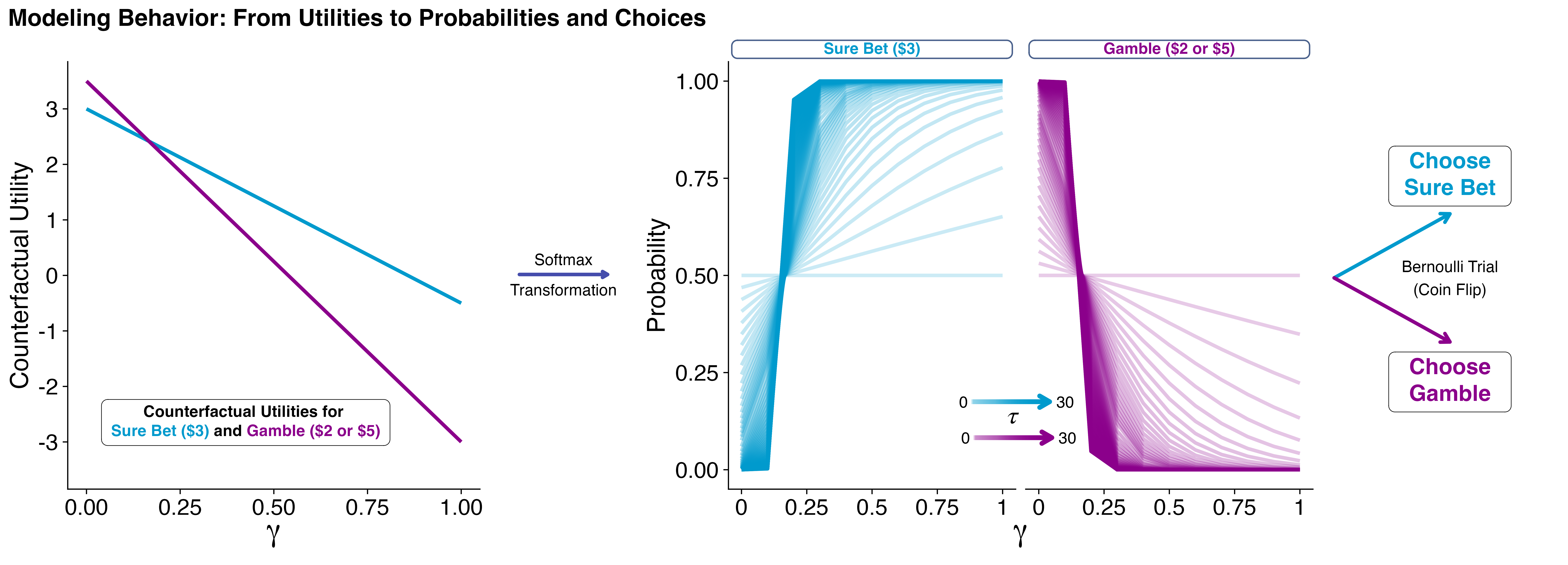
To build an intuition for how we can estimate the model’s parameters of interest, we can begin the ‘Simulation & Parameter Recovery’ step described in the chapter introduction. Figure 7.2 depicts the process of simulating a choice for the prospect included at the top of Figure 7.1. We first calculate counterfactual utilities for a prospect. Next, we apply the softmax choice rule to translate the utilities into a probability of choosing either option. Lastly, we ‘make’ a choice by flipping a weighted coin.

Figure 7.2: Depiction of the data generating process for modeling choice behavior with CPUT on the sure bet or gamble task. The left panel highlights the first step where counterfactual utilities are calculated. The middle panel shows the softmax transformation of the utilities into a probability of choosing either option; opacity of the logistic function increases with the softmax sensitivity parameter, \(\tau\), signaling a utility maximizing tendency. The right panel conveys how a choice is made by ‘flipping a weighted coin.’

When fitting a model on behavioral data, we assume that the statistical model represents how the data is generated. We can therefore work backwards by observing choices to infer the parameter values that are most plausible given the data. Bayes’ Theorem provides a way to update the most plausible parameter values for each choice observed.

To visualize a concrete example of this, I simulated nine choices between a sure bet of three dollars and a fifty-fifty gamble of two or five dollars (top panel from Figure 7.1) for an agent with \(\gamma = 0.25\) and \(\tau = 2.2\). For a given \(\tau\), our likelihood function assigns the probability of observing a choice for any \(\gamma\) value.

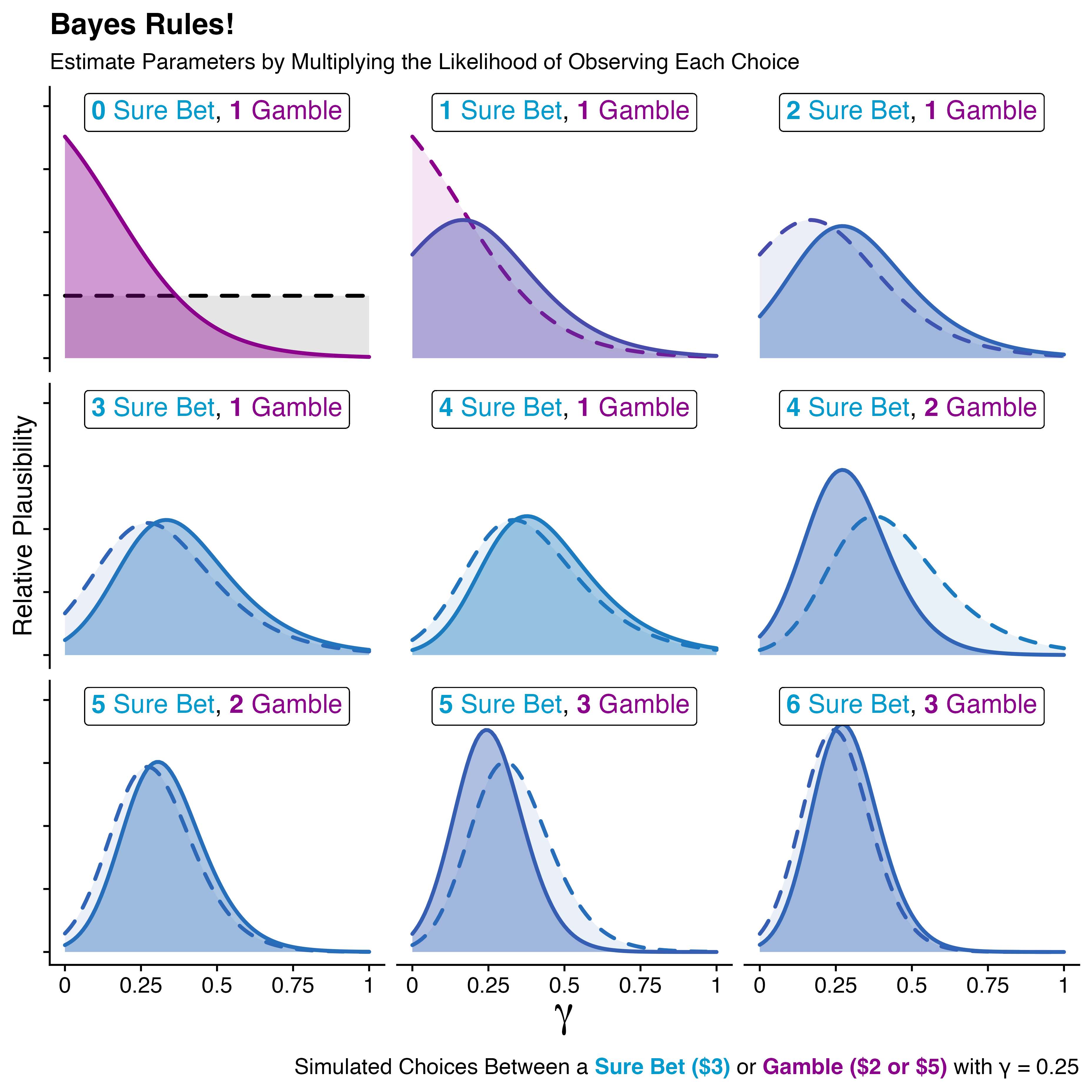
Consider the top left panel of Figure 7.3. Before observing any data, as specified in Equation (7.4), our prior (black, dashed line) is uniformly distributed between zero and one. The first choice our agent makes is a gamble. Multiplying our prior distribution for \(\gamma\) by the likelihood of choosing a gamble gives us the posterior plausibility for \(\gamma\) (purple, solid line). You may notice that the posterior distribution for this panel resembles the likelihood of choosing a gamble depicted in Figure 7.2. This is because the prior distribution for \(\gamma\) is initially uniform, so with one choice observed, the posterior plausibility becomes the likelihood.

This distribution becomes the starting point for future inference. In the next panel, our model observes a sure bet choice. Our most recent plausibility (purple, dashed line) is multiplied by the likelihood of observing a sure bet (depicted in Figure 7.2) to generate a new posterior distribution (blue-purple, solid line). This trend continues for each additional panel of Figure 7.3: our model observes a new choice and multiplies the likelihood of observing that choice by the previous posterior plausibility of \(\gamma\).

Figure 7.3: How a Bayesian model updates parameter estimates with new observations. Each panel shows a new choice simulated according to CPUT with \(\gamma = 0.25\). The model’s estimate of \(\gamma\) depicts the relative plausibility of each value. In each panel, most recent plausiblity (dashed line) is multiplied by the likelihood of observing the latest choice to produce the posterior plausibility (solid line).

Notice that each ‘sure bet’ choice shifts the range of plausible \(\gamma\) rightwards and each gamble choice shifts it leftwards. With each observation, the variance of the curve decreases, and the height increases. This highlights increasing evidence for the plausibility of \(\gamma\) values. As seen in the bottom right panel of Figure 7.3, we’re able to get an idea of the ‘true’ value of \(\gamma\) with relatively little data!

For this visualization, I fixed \(\tau = 2.2\), which made it easier to estimate the posterior probability of \(\gamma\). Simultaneously estimating multiple parameters often leads to computationally intractable posterior distributions, however. In the next section, I discuss a family of methods for efficiently calculating these joint posterior distributions known as ‘Markov Chain Monte Carlo.’

7.3 Posterior Estimation with Markov Chain Monte Carlo

For my thesis, I used two Markov Chain Monte Carlo methods. For the first, I manually implemented method is the Metropolis-Hastings algorithm in R.^[37,41] At a high level, it can be boiled down into three steps repeated for \(n \in 1:N\) iterations:

1. Propose a value, \(\theta_n^*\) near the current estimate \(\theta_n\), propose a value \(\theta^*\)
2. Calculate the acceptance probability for proposal \(\theta_n^*\) defined as the ratio between the posterior distribution evaluated at \(\theta_n^*\) to that of \(\theta_n\)
3. Draw a random number between zero and one. If it is less than or equal to the acceptance probability, set \(\theta_{n+1} = \theta_n^*\), otherwise \(\theta_{n+1} = \theta_n\).

I then validated my implementation by comparing it to posterior distributions computed with a hierarchical Bayesian approach. The Hierarchical Bayesian Analysis was implemented in the probabilistic programming language, Stan, which implements an efficient variant of Markov Chain Monte Carlo called the Hamiltonian Monte Carlo sampler.^[42] Hierarchical Bayesian Analysis allows for simultaneous estimation of individual and group-level parameters in a mutually-constraining fashion. This has been shown to improve parameter estimates relative to other methods (e.g., maximum likelihood estimation), resulting in more stable and reliable estimates for individual-level parameters as they are informed by group trends.^[43]

The specific implementation of hierarchical models I follow has been detailed elsewhere.^[44] At a high level, individual-participant parameters are assumed to be drawn from normally distributed group-level distributions. Bounded parameters, such as \(\gamma\), were estimated in an unconstrained space and transformed with the ‘Matt Trick,’^[42] an inverse Probit transformation. This is to optimize the MCMC sampling.^[44] More formally,

\[\begin{equation} \begin{aligned} \mu_\theta &\sim \text{Normal}(0,1) \\ \sigma_\theta &\sim \text{Half-Normal}(0,0.2) \\ \mathbf{\theta}^\prime &\sim \text{Normal}(0,1) \\ \mathbf{\theta} &= \text{Probit}^{-1}(\mu_\theta + \sigma_\theta \cdot \mathbf{\theta}^\prime) \times U.B. \end{aligned} \tag{7.5} \end{equation}\]

where \(- \infty < \mu_\theta < + \infty\) and \(- \infty < \sigma_\theta < + \infty\) are the group-level mean and standard deviation, respectively; \(\theta^\prime\) is the unconstrained parameter that gets transformed via the inverse Probit transformation and scaled to some upper bound, \(U.B\). As an example, for \(\gamma\), \(U.B. = 1\); for \(\tau\), \(U.B. = 30\). This non-centered reparameterization results in a uniform prior for individual participants’ parameters across the full range.^[44,45]

---

In this chapter, I hoped to provide an understanding of the computational modeling concepts used in my thesis. Specifically, I:

• Provided an overview of the sure bet or gamble task
• Mathematically described how we can estimate parameters from binary choice data using Bayes’ Theorem
• Visually depicted parameter estimation from choice data using Bayes’ Theorem for CPUT with simulated choices
• Introduced the Markov Chain Monte Carlo methods I use in my thesis to sample from the joint posterior distributions

With this foundation, it’s time to revisit the three computational modeling stages I introduced at the beginning of this chapter.^[36] Next, I outline my methods and results from simulating choice data according to counterfactual predicted utility theory, estimating parameters from observed data, and comparing evidence from three candidate models.