5 Neurobiology of Decision-Making

In the previous chapter, I used the term prospect to describe a problem that has two options with stated probabilities and outcomes. In the experimental literature, these prospects are called ‘description-based.’ Researchers who use description-based prospects in their experiments ask participants to select one of the available options that are presented along with a complete description of a non-trivial problem.^[9]

When looking towards the neuroscientific literature of decision-making, a different type of experimental paradigm is perhaps more common: ‘experiential’ or ‘feedback-based’ decisions.^[9]. By interacting with the environment, humans (and other animals) associate the consequences of different actions and adapt their behavior accordingly. In other words, we learn. We learn over time that we want to eat sushi for dinner, it’s faster to take the highway to work, and we’re better off if we go to sleep before midnight.³

That a behavior (an action or decision) is predicated upon prior experiences allows us to formalize the relationship between states. Here, I use state in reference to the representation of stimuli. For example, the state \(s \in S\) at time \(t\) (\(s_t\)) may be comprised of internal states (hunger, thirst, fatigue) or external ones (light, music, temperature).

Consider Pavlov’s experiment which showed how repeatedly giving a dog food after ringing a bell will condition the dog to salivate after the bell is rung.^[10] This means that, over time, behavior elicited by a stimulus (food) can be evoked by a previously neutral stimulus (the bell). In one of the first attempts to empirically describe this process, Bush and Mosteller suggest the probability of Pavlov’s dog salivating, \(P(\text{sal})\), on the next presentation of food with the bell (next trial, \(tr+1\)) is a function of what happened last presentation (last trial, \(tr-1\)) discounted by what was experienced during this presentation (food reward this trial, \(R_{tr}\).^[11,12]

\[\begin{equation} P(\text{sal})_{\text{tr}+1} = P(\text{sal})_{\text{tr}-1} + \alpha (R_{\text{tr}} - P(\text{sal})_{\text{tr}-1}) \tag{5.1} \end{equation}\]

Equation (5.1) computes an average of previously experienced rewards. \(0 \leq \alpha \leq 1\) is a learning rate, which modulates the influence of more recent rewards. Bush and Mosteller’s work forms the basis for modern approaches to this problem of reinforcement learning.^[13]4 While discretizing learning into trials is a logical first step to modeling behavior in experimental settings, it’s not easily applied to biological systems that continuously interact with their environments.

In his 1988 paper, Learning to Predict by the Methods of Temporal Differences, Richard Sutton introduces the antecedent for temporal-difference reinforcement learning (TDRL) algorithms.^[14] The TDRL algorithm provides a computational framework for optimally learning from experience how actions and their associated stimuli lead to rewards.^[15]

The ‘goal’ of TDRL algorithms is to estimate the value of a state and use that information to maximize rewards. This is achieved with a ‘teaching signal,’ called the temporal-difference reward prediction error (TD-RPE), which relates the value of being in a state at time \(t\) to what was expected previously.

This concept is perhaps best illustrated with an example. Imagine you order food from your favorite restaurant. You’ve tried every item on the menu, so you order your favorite dish.⁵ Because you’ve ordered it so much, you have a certain expectation about what the item smells like, how it tastes, and the state of contentedness you will feel after eating it.

We could represent the intrinsic value of eating the food at time \(t\) as \(V(S_t)\). To describe this in economic terms, this is the expected value of eating your favorite dish. Fortunately, the time has come, and your food is ready! You open the container and notice that something does not quite smell right. That is, your experience, \(\text{outcome}_t\), is negative. You expected a fragrant odor but were faced with something else. In other words, you expected something better than what you experienced. At the same time, your expectation of future enjoyment, \(V(S_{t+1})\) is still high. Maybe, you think, the odd smell comes from the container and not the food itself. Because of this, you remain hopeful for an enjoyable meal.

Each idea presented in the preceding paragraph is encapsulated by Equation (5.2) which defines the TD-RPE, \(\delta_t\), as the difference between the current value of a state at time \(t\) and what was expected. To summarize the notation:

• The value of a state is the sum of the experience (e.g., a displeasing odor, \(\text{outcome}_t\)) with the expectation of future values, \(V(S_{t+1})\). The value of future states are modulated by the temporal-discounting parameter \(0 \leq \gamma \leq 1\) which preferentially weights more immediate outcomes relative to future ones.⁶
• The expectation of a state, \(V(S_t)\), (e.g., an incredible culinary experience) is based on prior experiences.

\[\begin{equation} \delta_t = [\text{outcome}_t + \gamma V(S_{t+1})] - V(S_t) \tag{5.2} \end{equation}\]

On each time step, \(\delta_t\) is used to update the estimated value of the current state as formulated in (5.3).

\[\begin{equation} \hat{V}(S_t) \leftarrow V(S_t) + (\alpha \cdot \delta_t) \tag{5.3} \end{equation}\]

Whereas in Equation (5.1), the learning rate \(0 \leq \alpha \leq 1\) ascribed weight to recent rewards recently relative to those experienced in the more distant past. In contrast, the TDRL learning rate (also \(0 \leq \alpha \leq 1\)) controls how much weight an individual places on the estimated value of the current state in light of the TD-RPE. Put another way, it controls how much they update their future expectation given their most recent experience.

In the 1990s, Read Montague, Peter Dayan, and colleagues showed evidence suggesting that TD-RPEs are encoded by fluctuations in the activity of mesencephalic dopaminergic neurons.^[19,20] The implication that the dopaminergic system might encode TD-RPEs became known as TD-RPE hypothesis of dopamine neurons and is consistent with behavioral and neural results in rodents,^[21] non-human primates,^[22–25] and humans.^[26–29] Because of this biologically conserved mechanism for experiential learning, we can investigate the neural basis of choice behavior empirically with TDRL algorithms. In 2011, these experiments saw an exciting development when Ken Kishida and colleagues used fast-scan cyclic voltammetry to measure dopamine fluctuations in the human striatum with a sub-second temporal resolution.^[27]

In combination with their 2016 paper, Kishida and colleagues studied the dopamine levels of humans undergoing elective surgery as part of deep-brain stimulation treatment.^[27,30] Participants viewed a graphical depiction of a (fictitious) stock market’s price history (Figure 5.1; B) and were asked to choose how much of their portfolio (initially valued at $100) they would invest. For six ‘markets,’ each with twenty-decisions, participants used handheld button boxes (Figure 5.1; A) to increase or decrease their investment in ten-percent increments. Decisions were made in light of three pieces of information while sub-second changes in dopamine concentrations were recorded from the striatum:

1. The history of the market price (Figure 5.1; red trace in panel B)
2. The current portfolio value (Figure 5.1; bottom left box, 126, panel B)
3. The most recent fractional change in portfolio value (Figure 5.1; bottom right box, 15.2%, panel B).

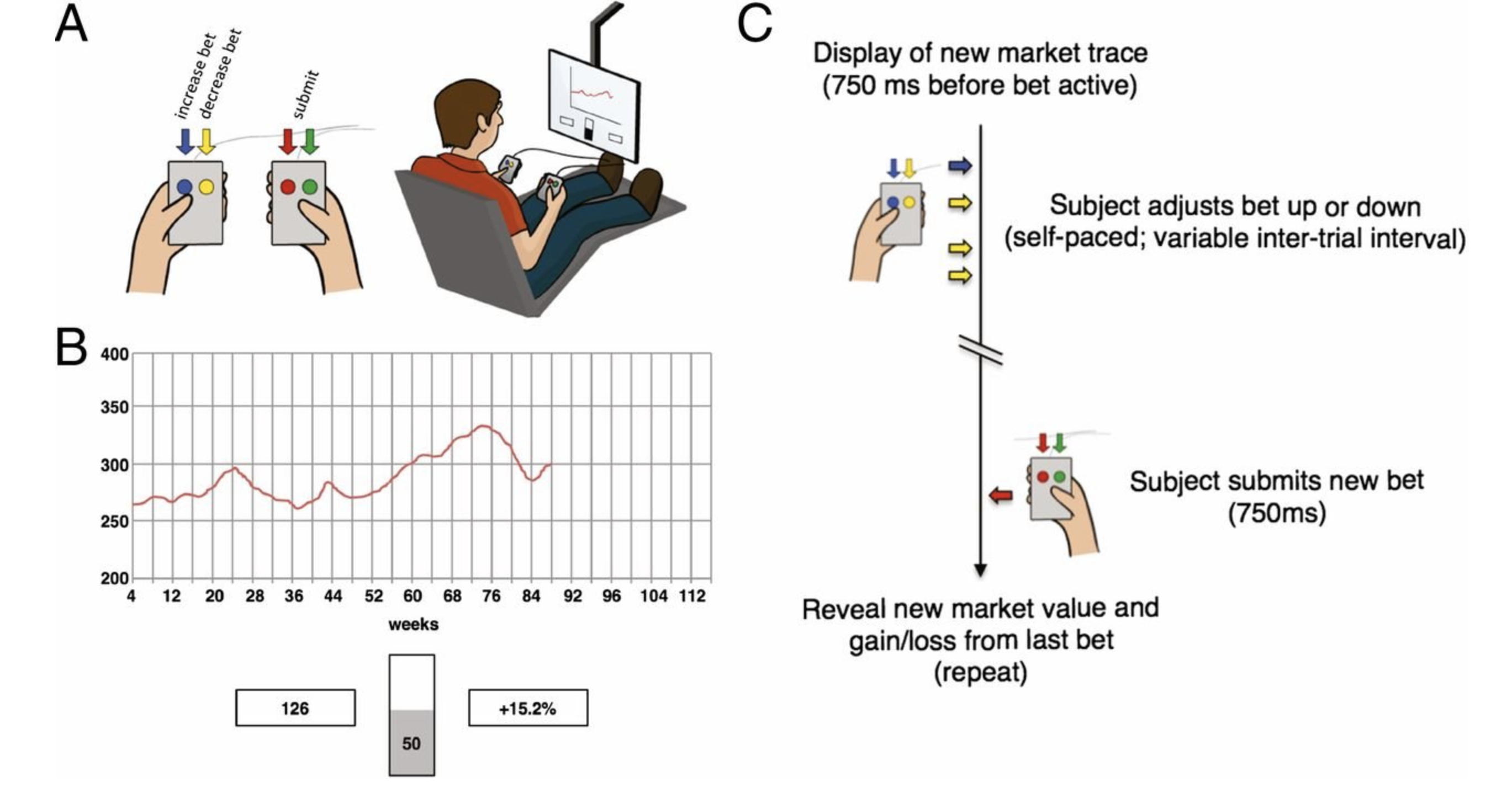
Figure 5.1: Participants played a sequential-choice game during surgery using button boxes (A; Left) and a visual display (A; Right). For each patient, bet size adjustments (e.g., increase bet or decrease bet) and the decision to submit one’s answer were performed with button boxes. (B) Graphical depiction of the market price history (red trace), their current portfolio value (bottom left box), and their most recent outcome (bottom right box) for sequential investment task. (C) Timeline of events during a single round of the investment game. Reprinted with permission from Kishida et al., 2016.

In their 2011 paper, they asked one person, MH, to complete the sequential investment task. In line with prior work relating dopamine with unexpected financial outcomes,^[26] Kishida and colleagues observed a strong correlation between MH’s dopamine levels and the market value during the investment task.^[27] In 2016, Kishida and colleagues published results from seventeen humans. Here, they explicitly tested the hypothesis that fluctuations in dopamine released in the human striatum encode TD-RPEs.^[30] For the sequential investment task, RPEs were calculated as the difference between an investment’s return on a given trial relative to the expectation defined by the average return from preceding trials.

Contrary to the hypothesis that dopamine fluctuations in the striatum should track TD-RPEs,^{[19,21,31–34]} the authors found that dopamine fluctuations encode an integration of RPEs with counterfactual prediction errors (CPEs). As discussed in the last chapter, counterfactual signals are an explicit comparison between the present state to alternative ones.^[7,8] For the sequential investment task, CPEs are defined as the difference between the participant’s actual return for a trial and what could have been had they invested more or less. This means that dopamine release is a result of the integration of RPEs and CPEs for a given trial. Formally:

\[\begin{equation} \begin{aligned} \text{dopamine transient} &\propto \text{RPE} - \text{CPE} \\ &\propto \text{RPE} - r_{tr}(1 - b_{tr}) \end{aligned} \tag{5.4} \end{equation}\]

where \(b_{tr}\) is the individual’s factional investment at trial \(tr\) and \(r_{tr}\) is the relative change in market price. As Kishida and colleagues note, the intuition for Equation (5.4) is that better-than-expected outcomes (positive RPEs, increased dopamine release), that could have been even better (positive CPEs) should be reduced in value. Similarly, worse-than-expected outcomes (negative RPEs, decreased dopamine release), that could have been even worse (negative CPEs) should be increased in value. Importantly, these empirical terms are consistent with the subjective feelings (e.g., regret and relief), one experiences in light of a given outcome.

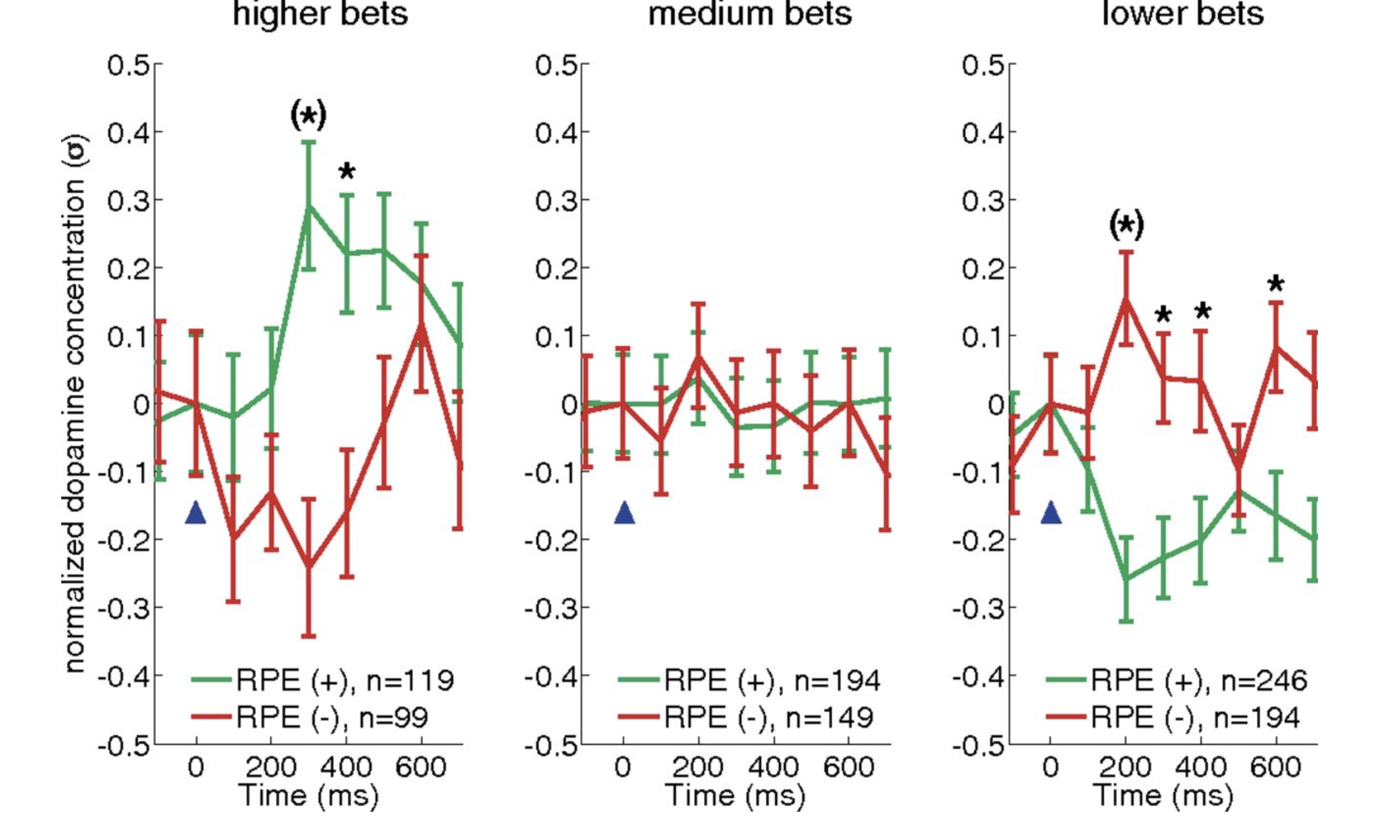
Figure 5.2: RPE encoding by dopamine transients invert as a function of bet size. Dopamine responses to equal absolute magnitude positive and negative RPEs when bets are high (Left), medium (Center), or low (Right). For all three plots, mean normalized dopamine responses with standard errors are shown for positive RPEs (green traces) and negative RPEs (red traces). Reprinted with permission from Kishida et al., 2016.

Figure 5.2 depicts changes in dopamine levels as a function of bet size. Consider the ‘higher bets’ panel (left) where individuals bet close to the maximum amount possible. When they were rewarded with a positive change in portfolio value, the dopamine concentrations increased (green; positive RPEs). Similarly, when the portfolio value decreased, dopamine levels dipped (red; negative RPEs). With high bets (left panel, bets between \(90\%-100\%\) of portfolio value), the difference between what they earned and what they could have earned had they bet more is minimal, as is the CPE. With medium bets (middle panel, \(60\%-80\%\)), however, the difference between what individuals experienced and what they could have experienced had they bet more increases. This means that the absolute magnitude of the CPE goes up which subtracts from the dopamine release predicted by positive and negative RPEs. When the CPEs are maximal (small bets, \(10\% - 50\%\); right panel), we observe an inversion in dopamine release in response to positive and negative RPEs.

The ‘superposed error signals about actual and counterfactual reward’ described in Kishida and colleagues’ paper^[30] directly inspired my thesis work. They provide an empirical, neurobiologically plausible framework for investigating decision-making under risk. The theoretical and quantitative underpinnings of classical and behavioral economic theories of decision-making align well with the computational reinforcement learning literature described in this chapter. The explicit probability and outcome structure for risky prospects afford the opportunity to internalize future states and (potentially) incorporate anticipated counterfactual events into the decision-making process. In the next chapter, I derive ‘Counterfactual Predicted Utility Theory’ as a new theory of decision-making under risk.