6 Counterfactual Predicted Utility Theory
As discussed in the neurobiology of decision-making chapter, the neurotransmitter dopamine seemingly encodes information about actual and counterfactual rewards,[30] and their integration may play a guiding role in decision-making. With this neural evidence, combined with behavioral economic theories offering descriptive models for people making risky decisions,[4,5] I propose ‘Counterfactual Predicted Utility Theory’ (CPUT) as a neurobiologically-plausible theory of decision-making under risk.
The impetus behind CPUT is the idea that people account for counterfactual outcomes when faced with a prospect and the integration of factual and counterfactual signals in the brain may discount or invert their preference for choosing one option over another. I hypothesize that this preference-reversal is modulated by a counterfactual weighting term, \(\gamma\), which may vary across people.
To formally derive CPUT, we can revisit the prospect I introduced in the first chapter with a hypothetical casino game. There are two options: choosing one will guarantee three-thousand dollars; choosing another will give you an 80% chance of four-thousand dollars or nothing. Such a prospect is commonly denoted as follows where the first option leads to outcome \(x_1\) with probability \(p_1\) and the second option leads to outcomes \(x_2\) with probability \(p_2\).
\[\begin{equation} \begin{aligned} \text{Option 1} &= (x_1, p_1) \\ \text{Option 2} &= (x_2, p_2) \end{aligned} \tag{6.1} \end{equation}\]Following conventional notation, the alternative outcomes of an option are assumed to be zero. That is, choosing Option 1 is a choice of receiving \(x_1\) with probability \(p_1\) or nothing with probability \((1 - p_1)\). This does not have to be true, however, and CPUT is formulated with a more generalizable representation of a prospect depicted in Figure 6.1. Here, Option 1 is a choice of receiving \(x_{1a}\) with probability \(p_1\) or \(x_{1b}\) with probability \((1 - p_1)\). Similarly, Option 2 is a choice of receiving \(x_{2a}\) with probability \(p_2\) or \(x_{2b}\) with probability \((1 - p_2)\).
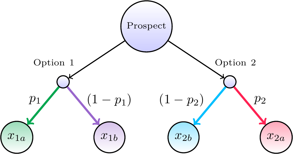
Figure 6.1: Explicit representation of a prospect with two options. Choosing option 1 may lead to outcome \(x_{1a}\) with probability \(p_1\) or outcome \(x_{1b}\) with probability \((1 - p_1)\). Choosing option 2 may lead to outcome \(x_{2a}\) with probability \(p_2\) or outcome \(x_{2b}\) with probability \((1 - p_2)\).
With this representation, we can begin to formally define an option’s counterfactual utility, \(U_C\), as follows:
\[\begin{equation} \begin{split} U_{C}(\text{Option 1}) = p_{1} \cdot V_{C}(x_{1a}) + (1 - p_{1}) \cdot V_{C}(x_{1b}) \\ U_{C}(\text{Option 2}) = p_{2} \cdot V_{C}(x_{2a}) + (1 - p_{2}) \cdot V_{C}(x_{2b}) \end{split} \tag{6.2} \end{equation}\]Similarly, we define Expected Utility as follows in Equation (6.3) which represents the same weighting as of probabilities and outcomes as Equation (6.2).
\[\begin{equation} \begin{split} U_{E}(\text{Option 1}) = p_{1} \cdot V_{E}(x_{1}) + (1 - p_{1}) \cdot V_{E}(x_{2}) \\ U_{E}(\text{Option 2}) = p_{2} \cdot V_{E}(x_{4}) + (1 - p_{2}) \cdot V_{E}(x_{3}) \end{split} \tag{6.3} \end{equation}\]The difference between the above equations is in the value estimates of each outcome. Expected Utility Theory exponentiates the stated outcome magnitude with a risk sensitivity parameter, \(\rho\).7 For CPUT, we define the transformation of the stated outcome as the face value minus a weighted sum of that option’s alternative outcome and the other option’s expected value. This notation is expressed in Equation (6.4), which shows how a prospect of the form depicted in Figure 6.1 are represented.
\[\begin{equation} \begin{split} \text{EUT:} \\ V_{E}(x_{1a}) = x_{1a}^\rho \\ V_{E}(x_{1b}) = x_{1b}^\rho \\ V_{E}(x_{2a}) = x_{2a}^\rho \\ V_{E}(x_{2b}) = x_{2b}^\rho \end{split} \hspace{3cm} \begin{split} \text{CPUT:} \\ V_{C}(x_{1a}) = x_{1a} - \gamma[x_{1b} + EV(\text{Option 2})] \\ V_{C}(x_{1b}) = x_{1b} - \gamma[x_{1a} + EV(\text{Option 2})] \\ V_{C}(x_{2a}) = x_{2a} - \gamma[x_{2b} + EV(\text{Option 1})] \\ V_{C}(x_{2b}) = x_{2b} - \gamma[x_{2a} + EV(\text{Option 1})] \end{split} \tag{6.4} \end{equation}\]Unlike the value estimate for Expected Utility Theory, \(V_E\), the estimated counterfactual utility value, \(V_C\) is not a one-to-one mapping of the stated outcomes. To provide a better intuition for this within- and between-option dependency, it is helpful to consider a concrete example. By adapting Figure 6.1 to include the values from the casino example initially described, we can better see how each possible outcome may integrate when evaluating a given prospect.
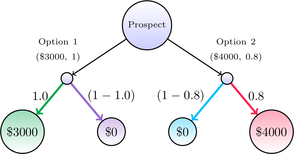
Figure 6.2: Example prospect diagram to visualize counterfactual integration. Choosing option 1 may lead to outcome \(\$3000\) with probability \(1.0\) or outcome \(\$0\) with probability \((1 - 1.0)\). Choosing option 2 may lead to outcome \(\$4000\) with probability \(0.8\) or outcome \(\$0\) with probability \((1 - 0.8)\). Estimating the counterfactual utility value of possible outcomes are dependent on one-another.
To illustrate CPUT by walking-through Figure 6.2, let’s assume that I have a counterfactual-weighting term of \(\gamma = 0.35\). This means that the stated outcomes are transformed given the available counterfactual information from each potential outcome as follows:
\[\begin{equation} \begin{aligned} V_{C}(\$3000) &= 3000 - 0.35[0 + EV(\text{Option 2})] \\ &= 3000 - 0.35[0 + 3200] \\ &= 1880 \\ V_{C}(\$0) &= 0 - 0.35[3000 + EV(\text{Option 2})] \\ &= 0 - 0.35[3000 + 3200] \\ &= -2170 \\ V_{C}(\$0) &= 0 - 0.35[0 + EV(\text{Option 1})] \\ &= 0 - 0.35[4000 + 3000] \\ &= -2450 \\ V_{C}(\$4000) &= 4000 - 0.35[4000 + EV(\text{Option 1})] \\ &= 4000 - 0.35[0 + 3000] \\ &= 2950 \\ \end{aligned} \tag{6.5} \end{equation}\]When these values are combined by Equation (6.2), we see that \(U_C(\text{Option 1}) > U_C(\text{Option 2})\):
\[\begin{equation} \begin{aligned} U_{C}(\text{Option 1}) &= 1 \cdot 2680 + (1 - 1) \cdot -620) \\ &= 1880 \\ U_{C}(\text{Option 2}) &= 0.8 \cdot 3700 + (1 - 0.8) \cdot -700) \\ &= 1870 \end{aligned} \tag{6.6} \end{equation}\]To maximize my utility, I would choose Option 1 and progress down the diagram to the first node on the left-hand side. In doing this, I forwent the opportunity to have Option 2. If I chose differently, I would have reached the node on the right, which has an expected value of $3200, but I didn’t. That is, the nodes on the right-hand side of the diagram are counterfactual events. By walking-through this example, I hope to convey how the possible outcomes relate to one-another and how factual and counterfactual information may be integrated to inform one’s decision.
Importantly, these equations suggest that when \(\gamma = 0\), when one places no weight on counterfactual events, the counterfactual utility is equivalent to the expected value. In other words, when \(\gamma = 0\), \(U_C(\text{Option 1}) = EV(\text{Option 1})\) and \(U_C(\text{Option 2}) = EV(\text{Option 2})\). If people don’t place weight on counterfactual information, we might expect choice behavior to be consistent with maximizing expected value (or, to better compare theories of decision-making, maximizing expected utility). To provide evidence in support of CPUT as a generative theory of decision-making, I will test the hypothesis that \(\gamma > 0\) which means that people do consider counterfactual outcomes when faced with a risky prospect.
To summarize what I discussed in this chapter:
- I addressed my first thesis aim of developing counterfactual predicted utility theory (CPUT) as an alternative to expected utility theory to explain decision-making under risk.
- I showed how information about each potential outcome (terminal node of Figure 6.1) integrates with a counterfactual weighting parameter, \(\gamma\), to adjust the utility of one option over another.
- I walked-through an example calculation assuming \(\gamma = 0.35\) (diagrammed in Figure 6.1).
In the next chapter, I begin to address my second thesis aim of assessing the descriptive and predictive validity of CPUT using human choice data from a ‘Sure Bet or Gamble’ task.[35]