8 Computational Modeling Methods and Results

Using the computational modeling techniques I introduced in the previous chapter, I examined the ability of counterfactual predicted utility theory to explain human choice behavior on the sure bet or gamble task.^[35] In this chapter, I present my methods and results concurrently following the three stages adapted from Wilson and Collins discussed in the introduction of Chapter 7.^[36] I start by simulating choice behavior generated from counterfactual predicted utility theory to confirm that the experimental design elicits behaviors assumed in the model. I then find estimate individual- and group-level parameters for three candidate models. Lastly, I quantify model fit with model comparison techniques.

8.1 Simulating Choice Data

As a first step to simulate choice data on the sure-bet or gamble task, I looked at the results of Kahneman and Tversky’s prospect theory^[4] paper in search of information to inform a prior distribution. Although there is no record for each subject’s response on specific prospects, Kahneman and Tversky report the proportion of people that chose each option. For each of the nine prospects that follow the form depicted in Figures 6.1 and 6.2, I used the reported proportions to simulate choice behavior of one-hundred subjects.

I assumed that $\gamma$ was uniformly distributed between zero and one and fixed the softmax sensitivity parameter, $\tau = 2.2$ following the conceptual visualizations from Section 7.2 consistent with the literature.^[39] I ran ten-thousand iterations using the Metropolis-Hastings algorithm described in the previous chapter. The posterior distribution, depicted in Figure 8.1, approximates a $\text{Beta}(1.1,1.1)$ distribution. This means that, in estimating $\gamma$ with the choice proportion data from Kahneman and Tversky, it’s plausible that $\gamma$ is any value between zero and one, though a little less likely towards the tails.

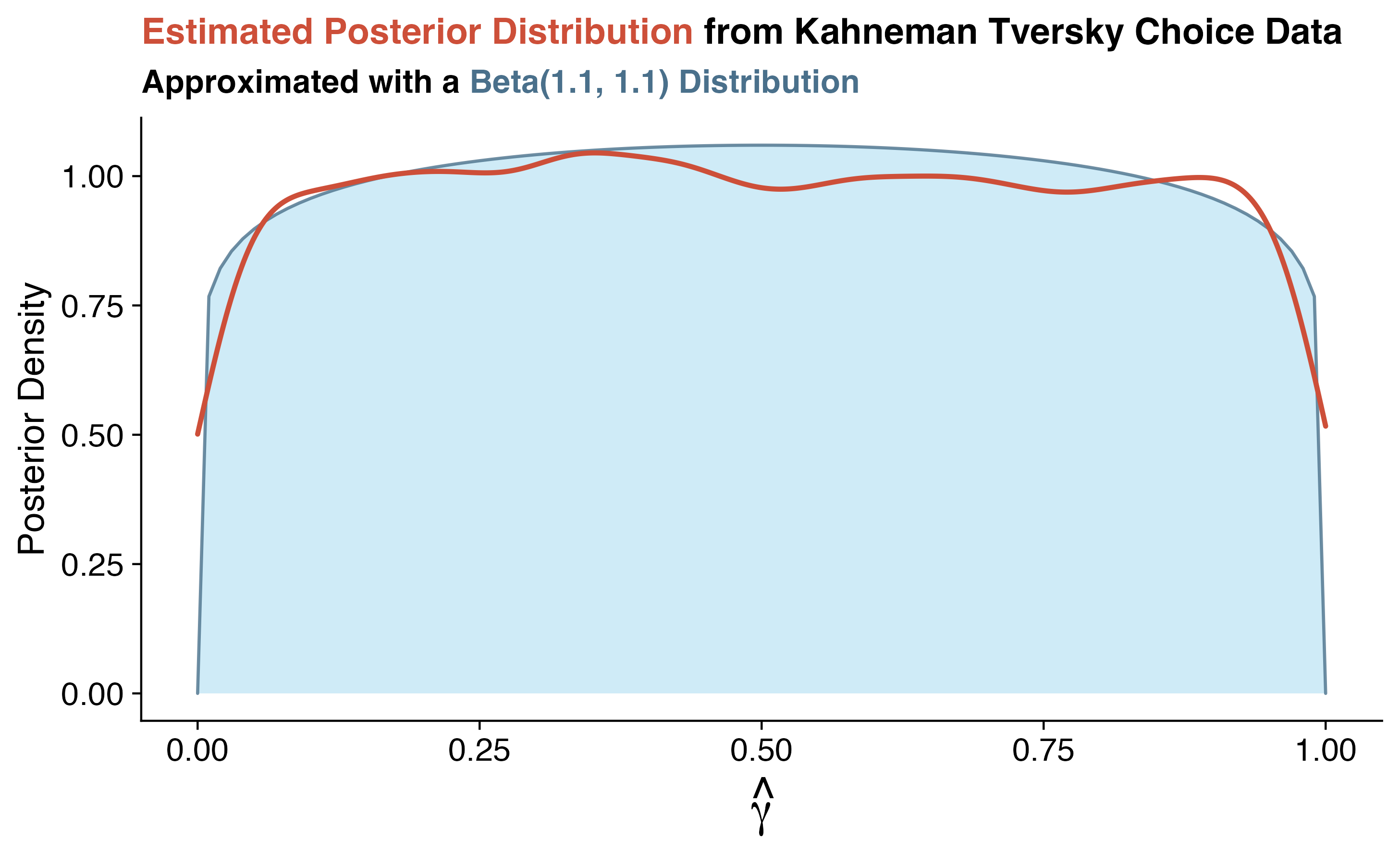
$Posterior distribution of $\gamma$ as estimated from ten-thousand iterations of a Metropolis-Hastings algorithm assuming a uniform prior with choice proportion data from Kahneman and Tversky's prospect theory. This posterior distribution (orange-red line) is approximated with a $\text{Beta}(1.1,1.1)$ distribution (blue-gray), indicating slightly less plausibility to $\gamma$ values near the bounds of the zero-to-one interval relative to central values.$

Figure 8.1: Posterior distribution of $\gamma$ as estimated from ten-thousand iterations of a Metropolis-Hastings algorithm assuming a uniform prior with choice proportion data from Kahneman and Tversky’s prospect theory. This posterior distribution (orange-red line) is approximated with a $\text{Beta}(1.1,1.1)$ distribution (blue-gray), indicating slightly less plausibility to $\gamma$ values near the bounds of the zero-to-one interval relative to central values.

Given the sure bet or gamble task design, participants saw a random subset of 252 prospects. The posterior distribution for $\gamma$ recovered from Kahneman and Tversky’s choice proportion data was used to generate $\gamma$ values for fifty subjects. I then simulated their choices on each of the 252 prospects, again fixing the softmax sensitivity parameter $\tau = 2.2$. For five-thousand iterations of the Metropolis-Hastings algorithm, I sampled from the posterior distribution for each simulated subject.¹⁰ With the same simulated data, I fit a hierarchical Bayesian model in Stan with the non-centered reparameterization as described in the computational modeling concepts chapter. I ran the Hamiltonian Monte Carlo (Stan) sampler for 5000 iterations across four parallel sampling chains for a total of 20,000 samples from the posterior.¹¹

I chose to estimate the posterior distribution with both the Metropolis-Hastings and Hamiltonian Monte Carlo algorithms to highlight the similarity in posterior parameter estimation techniques discussed in Chapter 7. Figure 8.2 shows the 95% highest density interval recovered from each sampler’s posterior distribution. For most subjects, the simulated $\gamma$ values are within the highest-density interval. This suggests that the sure-bet or gamble task is able to elicit the behaviors of interest in a way measurable with counterfactual predicted utility theory.

With the confirmation that I am able to accurately recover simulated parameters from the sure-bet or gamble task, I move on to the next stage of computational modeling, parameter estimation. To do so, I use the hierarchical Bayesian model in Stan for more stable and reliable estimates and computational efficiency.

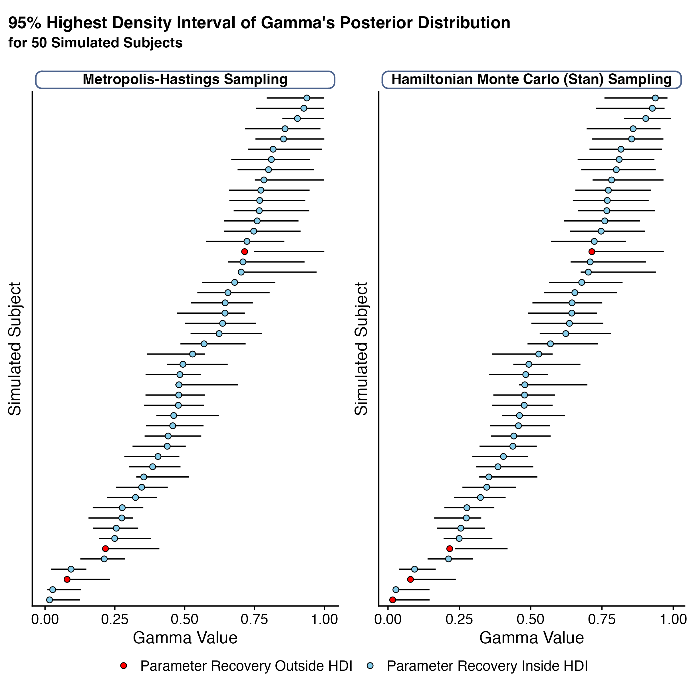
$95 percent highest density interval of the posterior distribution of $\gamma$ as estimated from five-thousand iterations of a Metropolis-Hastings algorithm and five-thousand iterations across four parallel chains with the Hamiltonian Monte Carlo Sampler (estimated using Stan). The simulated gamma values for each subject are represented as sky-blue dots if they fall within the highest density interval and red dots if they fall outside of it.$

Figure 8.2: 95 percent highest density interval of the posterior distribution of $\gamma$ as estimated from five-thousand iterations of a Metropolis-Hastings algorithm and five-thousand iterations across four parallel chains with the Hamiltonian Monte Carlo Sampler (estimated using Stan). The simulated gamma values for each subject are represented as sky-blue dots if they fall within the highest density interval and red dots if they fall outside of it.

8.2 Parameter Estimation

To assess counterfactual predicted utility theory’s validity as a theory of decision-making under risk, I estimate parameters for it in comparison with expected utility theory. I primarily do this for two reasons:

Counterfactual predicted utility theory suggests that, if $\gamma = 0$, the counterfactual utility of an option is equivalent to the expected value. The expected value is a special case of expected utility theory where the risk sensitivity parameter, $\rho = 1$.
The sure-bet or gamble task does not include losses, which prohibits me from comparing counterfactual predicted utility theory to prospect theory.

In addition to directly comparing CPUT with EUT, I wanted to see how different risk preferences might affect interact with counterfactual information to inform choice behavior. In total, I fit three models:

CPUT + Softmax Sensitivity: This model looks at how counterfactual information informs choice behavior. Its estimated parameters are the counterfactual weighting term, $\gamma$, and the sensitivity to differences in choice utilities, $\tau$.
CPUT + Risk Sensitivity + Softmax Sensitivity: This model looks at how differences in risk sensitivity may interact with counterfactual information to inform choice behavior. Its estimated parameters are the counterfactual weighting term, $\gamma$, the risk sensitivity term, $\rho$, and the sensitivity to differences in choice utilities, $\tau$.
EUT + Softmax Sensitivity: This model looks at how differences in risk sensitivity informs choice behavior. Its estimated parameters are the risk sensitivity term, $\rho$, and the sensitivity to differences in choice utilities, $\tau$.

All models were sampled for 5000 iterations across four parallel chains with the hierarchical Bayesian model formulation described in Section 7.3.^[44] For each model, chain convergence for group-level and transformed individual-level parameters was checked with Gelman-Rubin statistics, $\hat{R} \leq 1.1$, suggesting between-chain variance is lower than within chain variance.^[46] The group-level posterior distributions for parameters fit from each model are shown in Figure 8.3.

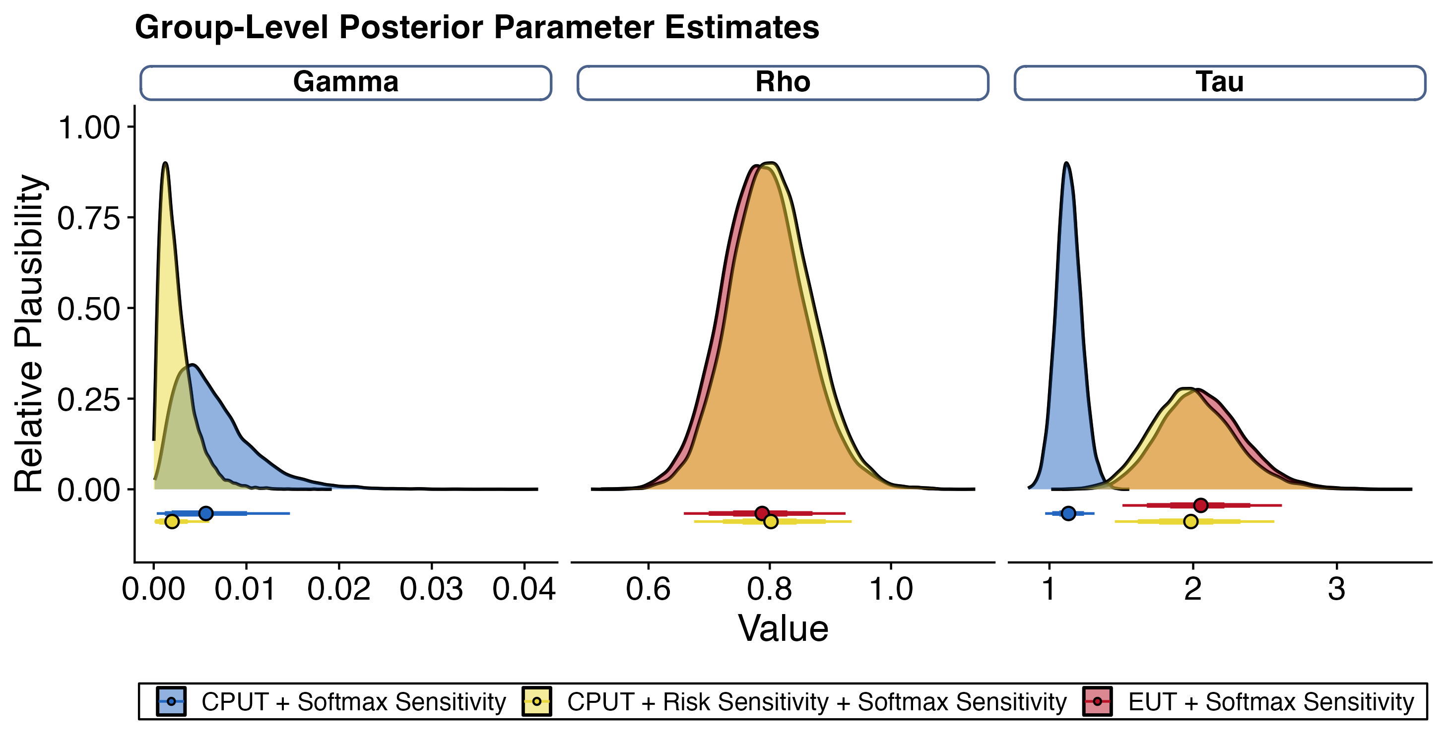
$Posterior distribution of group-level parameter estimates for each model. Relative distributions for $\gamma$ (left), $\rho$ (middle), and $\tau$ (right) underlined by 95 percent highest density intervals for each model with the median indicated. 'CPUT + Softmax Sensitivity' model shown in blue with estimated parameters for $\gamma, \tau$; 'EUT + Softmax Sensitivity' shown in red with estimated parameters for $\rho, \tau$; 'CPUT + Risk Sensitivity + Softmax Sensitivity' shown in yellow with estimated parameters for $\gamma, \rho, \tau$.$

Figure 8.3: Posterior distribution of group-level parameter estimates for each model. Relative distributions for $\gamma$ (left), $\rho$ (middle), and $\tau$ (right) underlined by 95 percent highest density intervals for each model with the median indicated. ‘CPUT + Softmax Sensitivity’ model shown in blue with estimated parameters for $\gamma, \tau$; ‘EUT + Softmax Sensitivity’ shown in red with estimated parameters for $\rho, \tau$; ‘CPUT + Risk Sensitivity + Softmax Sensitivity’ shown in yellow with estimated parameters for $\gamma, \rho, \tau$.

8.3 Model Comparison

With the estimated posterior distributions for each model type, I sought to determine which model best explains choice behavior. To do this, I used three different methods to compare models, the results of which are summarized in Table 8.4:

Posterior predictive checks where, for each model, I simulated choices given the (joint) posterior distribution of each participants’ estimated model parameter(s). This was included in Stan’s generated quantities block, which is only executed after a posterior sample has been generated.^[42] I then compared the percentage of predicted choices that matches the observed data and summarized the mean and standard deviation for each model.
Comparing the marginal likelihoods of each model. This is the probability of observing the choice behavior for a given model, $M$, $P(\text{Choices}|M)$. The marginal likelihood of each model was estimated using bridge sampling.^[47] Marginal likelihoods are often included in calculations of Bayes factors, which describes the relative evidence in favor of one model over another by quantifying the ratio between the probability of observing the data given two models. The marginal likelihoods are computed as log-scaled for computational efficiency, which means that the more positive, or less negative, marginal likelihood indicates a better fit.
Assessing penalized model fit with each model’s leave-one-out cross validation predictive accuracy.^[48] This is approximated with importance sampling of the posterior distribution to calculate the expected log pointwise predictive density (ELPD), which is the logged sum of pointwise posterior predictive distribution for held out data. By multiplying the ELPD by negative two, we get the leave-one-out information criterion, LOOIC. This transformation makes it easier to compare with other information criterion (e.g., AIC, DIC), highlighting the penalization of model complexity.^[49] I include both ELPD and LOOIC for easy comparison. Note that a less negative ELPD and a smaller (closer to zero) LOOIC are indicative of better model fits.

Parameters for, and description of, the different models fit on human choice data from the sure-bet or gamble task along with model comparison metrics. Posterior predictive choice accuracy represents the mean and standard deviation of correctly predicted choices for individual participants given simulations from the (joint) posterior distribution. ELPD Predictive Density and LOOIC details how well models perform on unobserved data (leave-one-out cross validation). Parantheses for ELPD and LOOIC indicate Monte Carlo sampling error. Marginal likelihood model evidence indicates the plausibility of the data given each model with parantheses representing the interquartile range of the likeihood estimations. In general, better models have smaller LOOIC and higher posterior predictive choice accuracy, ELPD predictive accuracy (less negative), and marginal likelihood model evidence (less negative). CPUT + Softmax Sensitivity and EUT + Softmax Sensitivity are highlighted for easy reference when discussed.

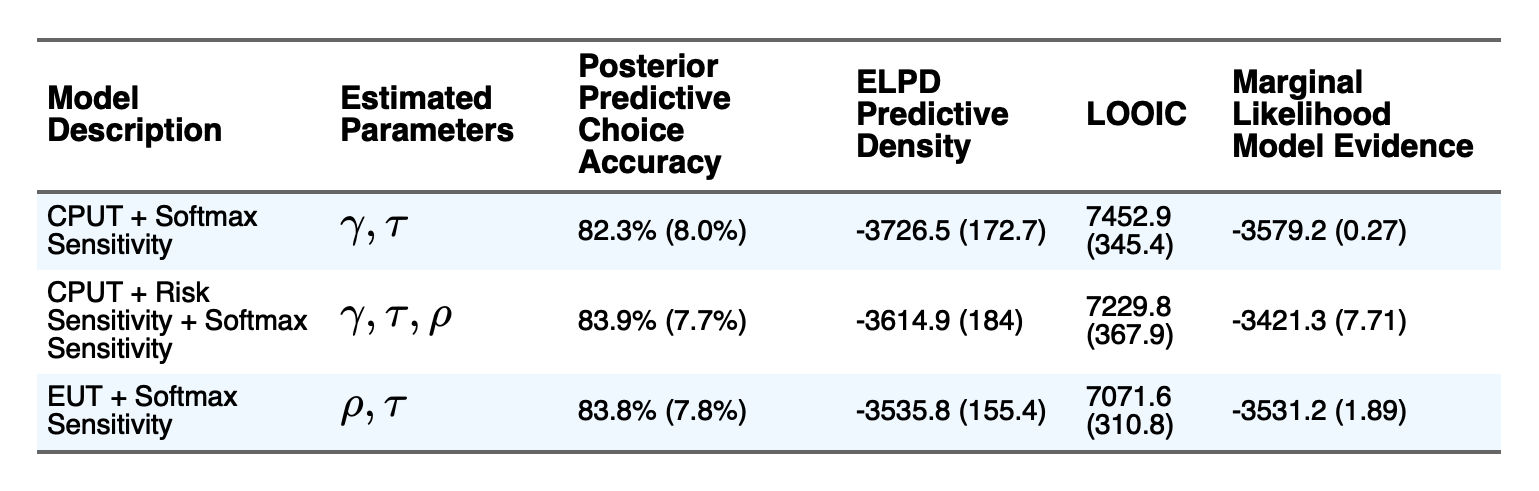
Figure 8.4: Parameters for, and description of, the different models fit on human choice data from the sure-bet or gamble task along with model comparison metrics. Posterior predictive choice accuracy represents the mean and standard deviation of correctly predicted choices for individual participants given simulations from the (joint) posterior distribution. ELPD Predictive Density and LOOIC details how well models perform on unobserved data (leave-one-out cross validation). Parantheses for ELPD and LOOIC indicate Monte Carlo sampling error. Marginal likelihood model evidence indicates the plausibility of the data given each model with parantheses representing the interquartile range of the likeihood estimations. In general, better models have smaller LOOIC and higher posterior predictive choice accuracy, ELPD predictive accuracy (less negative), and marginal likelihood model evidence (less negative). CPUT + Softmax Sensitivity and EUT + Softmax Sensitivity are highlighted for easy reference when discussed.

8.3.1 EUT versus CPUT

EUT provides a better explanation of the observed data on the sure bet or gamble task ($BF_{\frac{\rho, \tau}{\gamma, \tau}}$ = 48.07) and generalizes better than CPUT ($\text{LOOIC}_{\rho, \tau} - \text{LOOIC}_{\gamma, \tau}$ = -381.34). The posterior predictive choice accuracy – the percentage of choices simulated with the posterior estimate of each subject’s parameters – are similar, though better for EUT (83.8%) compared to CPUT (82.3%).

Further, the group-level posterior parameter distribution for $\tau$, the common variable to these two models, is higher for EUT than CPUT (95% HDI for EUT is [1.51, 2.62] with median of 2.05; CPUT = [0.97, 1.31] with median of 1.13). This suggests more utility maximizing decisions for EUT relative to more random choice behavior for CPUT.

8.3.2 CPUT + Risk Sensitivity versus EUT

Adding the risk sensitivity term, $\rho$, from EUT to CPUT offers the best explanation for the observed human choice data ($BF_{\frac{\rho, \tau, \gamma}{\rho, \tau}}$ = 109.89). This does come with a cost of decreased generalizability ($\text{LOOIC}_{\rho, \tau} - \text{LOOIC}_{\rho,\tau,\gamma}$ = -158.18) but increased posterior predictive choice accuracy (83.9% relative to EUT’s 83.8%).

Further, the group-level posterior parameter distribution for $\tau$ depict similar sensitivities to utility differences (95% HDI for ‘CPUT + Softmax + Risk Sensitivity’ = [1.45, 2.57] with median of 1.98; ‘EUT + Softmax = [1.51, 2.62] with median of 2.05) and risk sensitivity (95% HDI for ’CPUT + Softmax + Risk Sensitivity’ = [0.68, 0.94] with median of 0.8; ‘EUT + Softmax’ = [0.66, 0.93] with median of 0.79).

8.3.3 CPUT + Risk Sensitivity versus CPUT

Incorporating risk sensitivity to CPUT results in a better explanation for the observed data ($BF_{\frac{\rho, \gamma, \tau}{\gamma, \tau}}$ = 157.95), is more generalizable ($\text{LOOIC}_{\rho, \gamma, \tau} - \text{LOOIC}_{\gamma, \tau}$ = -223.16), and has a higher posterior predictive choice accuracy (83.9%) relative to CPUT’s (82.3%).

Interestingly, the group-level posterior parameter distribution for $\tau$ with the CPUT + Risk Sensitivity more closely reflects that of EUT. At the same time, the group-level posterior parameter distribution for $\gamma$ is much more tightly concentrated towards zero than for CPUT (95% HDI for CPUT + Risk Sensitivity is [<0.001, 0.006] with median of 0.002; CPUT = [<0.001, 0.015] with median of 0.006). This suggests more a lower weighting on counterfactual information while accounting for risk preferences.

By most measures, it seems that Expected Utility Theory provides the most generalizable explanation of human choice data on the sure bet or gamble task. In the next chapter, I discuss these results and outline next steps to contribute towards a better understanding of the neurobiological basis of decision-making under risk.

7 Computational Modeling Concepts

9 Discussion & Next Steps